
![A sculpture commemorating one of the greatest physicists in the 20th century, Paul Dirac, it stands on the Anchor road in front of Bristol cathedral, next to where I work. [1]](/images/2023-02-09-smoothed_particle_hydrodynamics/paul_dirac_monument.png)
“No matter how hard you squeeze your fist, there always is a gap in the atomistic scope.”
I was so fascinated by this phenomenon when a physics teacher told us about intermolecular forces in middle school, that is, particles of matters attract each other within a certain range and push each other away when they are too close. This simple idea has helped me to conceptualise how Smoothed Particle Hydrodynamics(SPH) works. Particles will act and react to its surrounding particles, the closer they are, bigger the influence.
SPH is a numerical discretisation method, and should not be confused as one of Computational Fluids Dynamics(CFD) methods. It is true that SPH has many applications in fluids simulation and widely used in computer graphics community. And it can be derived to many forms to solve partial differential equations such as the Euler equation(inviscid fluids) and Navier-Stoke equation in a lagrangian system. However, it was originally designed for astrophysical simulation, and later served as an approximation method in continuum mechanics. More importantly, SPH has strong theory supports, researchers have been working for decades to provide mathematical soundness and robustness of SPH.
In this post, I will introduce the basic math of SPH and how it works.
 Fluid simulation using SPH[2]
Meaning of SPH
The “Smoothed Particle Hydrodynamics” method consists of 3 terms that reveal the quintessence of its ideology and functionality. The ‘SMOOTHED’ term indicates the method uses a smooth kernel function to approximate a point of interest using its local neighbouring particles with different weights. ‘Particle’ specifies it is a Lagrangian mesh-free particle method. ‘Hydrodynamics’ means this method is designated for applications in continuum mechanics problems.
Function Approximation
The properties of a continuous field such as density, velocity, and pressure can be expressed as a set of PDEs. To solve the PDEs, we need to find the integral representation of the continuous function. We can estimate a function’s integral in an infinitesimal range by calculating the area beneath the curve. The mean value theorem equips us with a nice integral representation so the integral value at any point can be calculated. 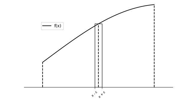 Mean Value Theorem for Integral Representation
where the $\delta(X-X’)$ is the well known Dirac-Delta function, The delta function has to meet the condition that $\int \delta\left(X -X’\right)dX’ = 1$ for the equation to be an exact solution, it is also know as the normalisation(unity) condition. There are a few more important conditions the smoothing function has to meet will be discussed later.
In SPH, the Dirac-Delta function is replaced by a smooth function so an approximation model can be computed. The smooth function with finite support to approximate the function can be written as follows:
\[<f(X)>=\int_{\Omega} f\left(X^{\prime}\right) W\left(X-X^{\prime}, h\right) d X^{\prime}\]where $<f(X)>$ is the approximate value of the function at the position X, $<f(X)>$ is often written in $f(X)$ for simplicity, $f(X^{\prime})$ is the value of the function in the position of the neighbouring points. $W\left(X_{i}-X_{j}, h\right)$ is the kernel weights evaluated at the position $X^{\prime}$ based on the distance between $X$ and $X^{\prime}$. The conditions for construction of kernel function are introduced in later section.
A vectorial function f has spatial derivative of $\nabla f$. Then the arbitrary function can be written as in the form of SPH approximation:
\[\nabla f(X)=\int_{\Omega}\left[\nabla f\left(X^{\prime}\right)\right] W\left(X-X^{\prime}, h\right) d X^{\prime}\]The differential operations are linear operators, thus it obeys following product rule:
\[\nabla (\varphi f)=\varphi \cdot (\nabla f) + (\nabla \varphi) \cdot f\]Therefore, the term at the right side of the derivative equation can be written as:
\[\nabla f\left(X^{\prime}\right) W\left(X-X^{\prime}, h\right)=\nabla f\left(X^{\prime}\right) \cdot W\left(X-X^{\prime}, h\right) -f\left(X^{\prime}\right) \cdot \nabla W\left(X-X^{\prime}, h\right)\]Split the integration part of the derivative Equation, we get:
\[\nabla f(X)=\int_{\Omega} \nabla f\left(X^{\prime}\right) \cdot W\left(X-X^{\prime}, h\right) d X^{\prime}-\int_{\Omega} f\left(X^{\prime}\right) \cdot \nabla W\left(X-X^{\prime}, h\right) d X^{\prime}\]Applying the divergence theorem, we get an equivalent equation as:
\[\nabla f(X)=\int_{s} f\left(X^{\prime}\right) W\left(X-X^{\prime}, h\right) \mathbf{n} \cdot d \mathbf{S}-\int_{\Omega} f\left(X^{\prime}\right) \cdot \nabla W\left(X-X^{\prime}, h\right) d X^{\prime}\]Since the kernel function is compactly supported, the local domain surface integral is assumed to be zero, thus the derivative equation can be express in the term of function value and derivative of the smooth function only:
\[\nabla f(X)=-\int_{\Omega} f\left(X^{\prime}\right) \nabla W\left(X-X^{\prime}, h\right) d X^{\prime}\]Similarly, we can obtain the divergence approximation by:
\[\nabla \cdot f(X)=-\int_{\Omega} f\left(X^{\prime}\right) \cdot \nabla W\left(X-X^{\prime}, h\right) d X^{\prime}\]The Laplacian of a function is defined as a second-order differential operation. It is defined as the divergence of the gradient of the function:
\[\Delta f=\nabla^{2} f=\nabla \cdot \nabla f\]Thus, using the same technique we can obtain the Laplacian approximation as:
\[\Delta f(X)=-\int_{\Omega} f\left(X^{\prime}\right) \cdot \Delta W\left(X-X^{\prime}, h\right) d X^{\prime}\]Generally, higher-order derivatives can be repeatedly derived using mathematical derivations from their previous order equations recursively. A first-order accuracy is proven when more properties of the smoothing function are introduced.
Function Discretisation
A continuous form of functions and their derivatives are phrased in integral representations. For computers to solve the numerical scheme, accurate discretisations are required. In SPH, the discretisation method is also called particle approximation. The computational domain is a collection of discrete particles with physical properties, and each particle is evaluated and summed by neighbouring particles. Since the Dirac-Delta function would model an idealised point mass with no spatial extents, thus the mass can not be computed as the spatial integral from density. The infinitesimal spatial extents $dX^{\prime}$ will have to be replaced by a $\Delta V$. Hence the mass can be modelled as:
\[m = \int \rho(X)dV\]Therefore, the discretisation of the kernel approximation are procured from integration form of SPH approximation:
\[\begin{aligned} f(X) &= \int_{\Omega} f\left(X^{\prime}\right) W\left(X-X^{\prime}, h\right) d X^{\prime} \\ & \approx \sum_{j=1}^{n} f(X_{j}) W\left(X-X_{j}, h\right) \Delta V_{j}\\ & = \sum_{j=1}^{n} f(X_{j}) W\left(X-X_{j}, h\right) \frac{m_{j}}{\rho_{j}} \\ & = \sum_{j=1}^{n} \frac{m_{j}}{\rho_{j}} f(X_{j}) W\left(X-X_{j}, h\right) \\ \end{aligned}\]In a similar fashion, the continuous derivatives equations can be written as:
\[Gradient: \nabla f(X) = \sum_{j=1}^{n} \frac{m_{j}}{\rho_{j}} f(X_{j}) \nabla W\left(X-X_{j}, h\right)\] \[Divergence: \nabla \cdot f(X) = \sum_{j=1}^{n} \frac{m_{j}}{\rho_{j}} f(X_{j}) \cdot \nabla W\left(X-X_{j}, h\right)\] \[Laplacian: \Delta f(X) = \sum_{j=1}^{n} \frac{m_{j}}{\rho_{j}} f(X_{j}) \Delta W\left(X-X_{j}, h\right)\]where $ \nabla W\left(X-X_{j}, h\right)$ is often simplified as $ \nabla W_{ij}$ and $\nabla W_{ij} = \frac{X_i - X_j}{r_{ij}}\frac{\partial W_{ij}}{r_{ij}} = \frac{X_{ij}}{r_{ij}}\frac{\partial W_{ij}}{r_{ij}}$, $r_{ij}$ is the scalar distance between two points.
And above equations are the basis of SPH numerical scheme, we have all these discretisation tools to solve a partial differential equation.
Smoothing functions conditions
Smoothing functions is sometimes named kernels in approximation theory. The smoothing functions should be at least twice continuous differentiable due to the formulation in SPH. Going back to the integral representation of the SPH formulation, the errors can be analysed by Taylor series expansion:
\[\begin{split} f(X) &= \int f\left(X^{\prime}\right) W\left(X-X^{\prime}, h\right) d X^{\prime} \\ &= \int [f(X) + \nabla f(X - X^{\prime}) + \frac{1}{2}(X - X^{\prime}) \cdot \nabla^{2}f(X - X^{\prime}) + O((X - X^{\prime})^{3})] W\left(X-X^{\prime}, h\right) d X^{\prime} \\ &= f(X) \int W\left(X-X^{\prime}, h\right) dX^{\prime} + \nabla f(X) \int (X-X^{\prime}) W\left(X-X^{\prime}, h\right) dX^{\prime} + O((X - X^{\prime})^{2})\\ \end{split}\]The normalisation/unity condition for smooth functions is inherited from the Dirac-Delta function, which makes the integral in the first term of the above equation conveniently become 1. To make the approximation $1^{st}$ order accurate, a symmetric property can be introduced to smooth functions, so that the integral in the second term in the taylor series will be cancelled out to zero. Other properties are summarised as follows:
Normalisation/Unity: $\int W(X-X^{\prime}) dX^{\prime} = 1$. This is one of the most important requirements for smoothing functions so that the integral of the kernel in the local domain is normalised.
Symmetric: $W(X-X^{\prime}) = W(X^{\prime} - X)$. As proven previously in the Taylor expansion analysis, the Symmetric property is necessitated to ensure $1^{st}$ order accuracy.
Compact support: $W(X-X^{\prime}) = 0$, if $ \left\lvert X-X^{\prime} \right\rvert> kh $, where h is the support radius length and k is an arbitrary scaling factor. In SPH approximation, compact support allows the kernels only convolve only the support domain and eliminate the influence of discrete particles from far in the global domain, which guarantees the local accuracy for sparse particle modelling. Compactness also provides the SPH adaptability to neighbourhood search algorithms for efficient computing.
Delta function property: $\lim _{h \rightarrow 0} W (X-X^{\prime}, h )=\delta (X-X^{\prime})$. As the support radius tend to zero, the discrete approximation should be equal to the continuous integral representation.
Positivity:$W(X-X^{\prime}) \ge 0$. Positiveness ensures that the physical properties of particles remain meaningful, such as the density should always keep positive for a stable simulation.
Decay: The weights computed by the smoothing function should monotonically decrease due to the consideration that further particles should have less physical effects on centre points.
Smoothness:: The smoothing functions needs to be sufficiently smooth until the second order for an accurate approximation for gradient and Laplacian terms. The smoothness and continuousness in the derivatives greatly impact numerical results and their stability.
 Gaussian kernel with cutting off condition
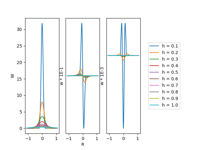
An obvious selection of kernels would be using the normalised Gaussian function:
\[W\left(X_{i}-X_{j}, h\right) = W(R, h)=\alpha_{d} e^{-R^{2}}\]The Gaussian kernel is twice continuously differentiable and has a sufficient enough smoothness for second-order derivatives. Though it is really not compactly supported since as the further distance, the weights will approach zero but never reach zero.
Benchmark Result
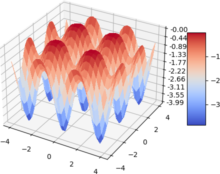
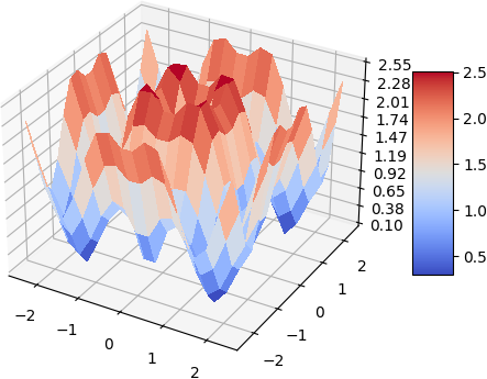
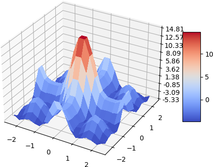
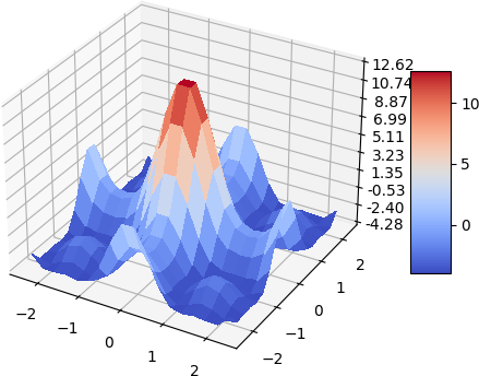
A quick demo of approximate a simple 2d function and its gradient and laplacian is demonstrated below, 900 data points are used, some randomness of the collation points are also added. the test function used is:
\[f(x, y) = -(cos^2(x) + cos^2(y))^2\]| Analytical | Approximation |
|---|---|
 | 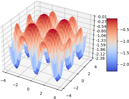 |
Gradient
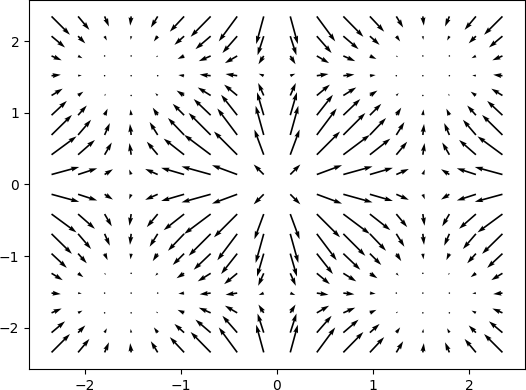 | 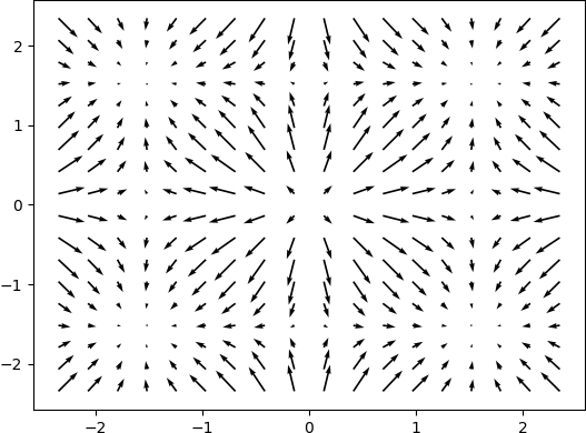 |
Magnitude of Gradient
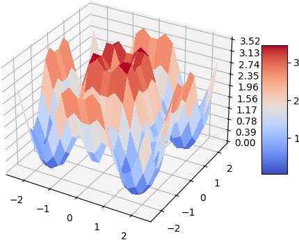 |  |
Laplacian
 |  |
Recommended literature
My favorite piece of introduction to SPH is the Eurographics tutorial by Bender and Koschier, which is a very good starting point for beginners. They are the authors of the open source SPH library SPlisHSPlasH. This review by Lind is a very well written and comprehensive introduction to SPH flow modeling, which is a good reference for further reading. Introduction from the father of SPH Monaghan and slightly more advanced introduction from Price are also very nice reads.
fro fluid simulation, the recommended sequence is: WCSPH -> PCISPH -> IISPH -> DFSPH
Books I like:
- <Smoothed Particle Hydrodynamics - Fundamentals and Basic Applications in Continuum Mechanics>, Carlos Alberto Dutra Fraga Filho
- <Smoothed Particle Hydrodynamics: A Meshfree Particle Method>, G. R. Liu
Reference
[1] Farmelo, The Strangest Man: The Hidden Life of Paul Dirac, Quantum Genius, 2009.
[2] An open source software provide simulations based on SPH, SPlisHSPlasH.